Four Days of RL: One Gradient, Dressed Four Ways

Reinforcement learning was the part of modern AI that looked most alien from where I sit. I build data pipelines. Supervised learning I can map onto my day job: data in, labels in, model out. RL looked like a different religion.

So I spent four days on foundations: David Silver’s DeepMind lectures, Stanford’s CS224R, Sutton and Barto, and a build every single day, because watching videos without typing is how you convince yourself you understand something you don’t. The code for all four days is on GitHub. This post is what stuck, and the one idea that reorganized everything: there is basically one gradient in this whole field, and everybody is arguing about how to dress it.

I am ramping toward a longer build I’ll write about soon. This is the floor it stands on.

Table of contents

Day 1: The loop you should be able to write from memory

Nothing in RL is learnable if the PyTorch training loop still requires thinking. So day one was pure fluency: the official tutorials end to end, a FashionMNIST MLP, and then the exercise that actually taught me something. Close everything. Blank file. Rewrite the whole pipeline from memory. I failed partway, peeked, finished, and did it again the next morning as a warm-up. By day three I could type it while thinking about something else, which is the point.

The distilled skeleton is committed with every line commented in my own words. The spine never changes:

for epoch in range(epochs):
    for X, y in dataloader:
        optimizer.zero_grad()
        pred = model(X)
        loss = loss_fn(pred, y)
        loss.backward()
        optimizer.step()

Zero the gradients, forward, score, assign blame backward, step. Every algorithm in the next three days is this loop with a different opinion about where loss comes from.

Day 2: Bellman is a fixed-point computation

Day two was the problem statement. An agent in a state takes an action, the environment returns a reward and a next state, repeat. The goal is a policy that maximizes cumulative discounted reward. Fine. The idea that made it click was the Bellman equation, which sounds imposing and is actually one sentence: the value of a state is the best immediate reward plus the discounted value of wherever you land.

That sentence is recursive, and recursive definitions get solved by iteration. I built a 4x4 gridworld in pure NumPy, minus one reward per step, goal in the corner, and implemented value iteration: sweep every state, apply the Bellman update, repeat until nothing changes.

while True:
    delta = 0
    for state in all_states:
        best = max(reward + GAMMA * V[next_state]
                   for each action)
        delta = max(delta, abs(best - V[state]))
        V[state] = best
    if delta < THETA:
        break

If you have ever run an iterate-until-convergence graph job, Pregel-style, you have already run this algorithm. Same shape: propagate a number through neighbors until the largest change drops below a threshold. Watching the printed value grid evolve, you can see value flow backward from the goal, one sweep at a time, exactly the way shortest-path distances flow outward from a source. Planning, it turns out, is a fixed-point computation over a graph. I do those for a living.

Two things from the Silver lectures earned a permanent place in my notes. First, the reward hypothesis, which the whole field quietly stands on: every goal can be described as maximization of expected cumulative reward. Every goal. You can accept it or fight it, but the entire edifice assumes it. Second, the discount factor has three separate justifications that all give the same answer: the math needs it to converge, the future is genuinely uncertain, and, well, animals discount too. When theory, uncertainty, and biology agree on a constant, use the constant.

Day 3: Watching supervised learning fail on schedule

Day three is the day CS224R sets a trap for you, and the trap is the lesson. The most obvious way to teach a policy is to skip RL entirely: record an expert, then train a classifier from states to actions. Behavioral cloning. It’s supervised learning wearing a trench coat.

I wrote a ten-line heuristic expert for CartPole, push toward the pole’s lean, collected 50 expert episodes, and trained a two-layer MLP to imitate it. The clone learns the mapping almost perfectly on its training data. Then you run it, and this happens:

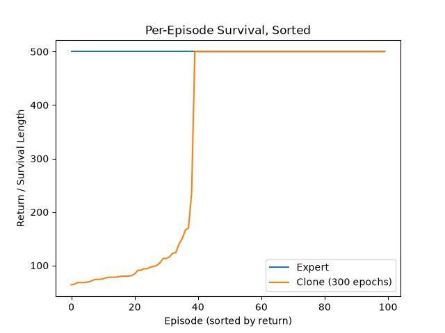
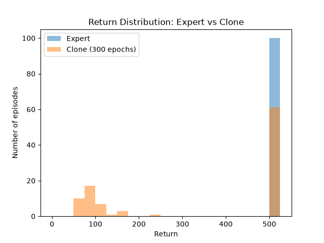
Those are my actual evaluation plots, 100 episodes each. The clone tracks the expert on easy episodes and dies early on a chunk of the rest. The mechanism is the important part. The clone was trained only on states the expert visits. One small mistake nudges it into a state the expert never showed it, where its behavior is undefined, so it errs again, drifts further, and compounds. The failure is not noise. It is structural.

Data engineers have a name for the general disease: training-serving skew. The distribution you trained on is not the distribution you serve on. What makes the RL version vicious is that the skew is self-inflicted, the model’s own actions generate the out-of-distribution states. It is a feedback loop wearing a distribution-shift costume. DAgger, the classic fix, is exactly what a data engineer would invent: go label the states the learner actually visits, not the states the expert prefers, and retrain. Fix the sampling, fix the model.

Day 4: The keystone

Day four is the reason the other three exist. If imitation compounds errors, learn from reward directly. But there’s an obstacle that defines the whole field: the environment is not differentiable. You cannot backprop through a physics engine, a market, or a patient. The reward comes out of a black box.

The escape is the score-function trick, and it is the single most important idea of the four days. You cannot differentiate the world, but you can differentiate the one thing you own: the probability your policy assigned to each action it took. Multiply each action’s log-probability by how well the episode went, and push probability toward actions from good episodes.

returns = discounted_returns_to_go(rewards, gamma)
loss = -(log_probs * returns).sum()
loss.backward()
optimizer.step()

That is REINFORCE, and it drops straight into the day-one skeleton. Look at it long enough and it resolves into something familiar: cross-entropy where every label is weighted by how the story ended. Actions from a 500-step episode get reinforced hard. Actions from a 20-step faceplant get suppressed. Supervised learning, except the labels are graded by outcome.

It works, and it is noisy, because a whole episode’s return is a high-variance judge of any single action. The first fix is subtracting a baseline, and it comes with the best free lunch in the field: subtracting any state-dependent baseline changes nothing in expectation, E[grad log pi times b] is exactly zero, but it collapses the variance. I trained CartPole to the standard solved bar, average return above 475 across 100 evaluation episodes, and the baselined version gets there with visibly calmer learning curves.

Here is where the four days compound into one picture:

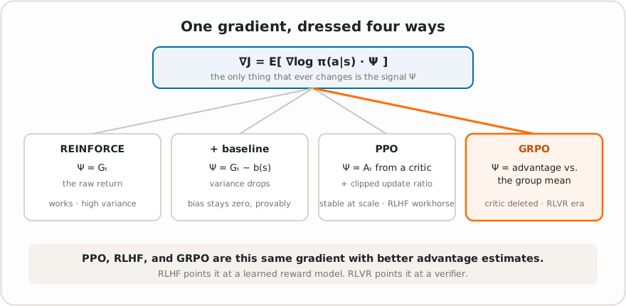
Everything in modern post-training is this gradient with a better-behaved signal in the middle. Add a learned critic and a clipped update ratio, that’s PPO, the workhorse of RLHF. Point the gradient at a learned reward model, that’s RLHF itself. Delete the critic and use the group mean of sampled completions as the baseline, that’s GRPO, the algorithm behind the current reasoning-model wave. The five lines above are the ancestor of all of it.

What this sets up

Four days bought me the thing I actually needed: the ability to read a post-training paper and see the skeleton under the clothes. The gradient never changes. The signal does. Which raises the question the whole field is currently organized around: where does a trustworthy signal come from?

The most interesting answer right now is: from a verifier. A program that checks the output. Put a verifiable reward where G used to be and the noisy episode-return problem becomes a precision instrument. That is the direction I’m building in next.

The gridworld, the cloning experiment, and the plots are all in the repo. Day 5 was policy iteration’s smarter siblings. But that’s another post.